Many real-world systems, like El Niño-Southern Oscillation (ENSO) or glucose fluctuations in patients with type-1 diabetes, tend to shift their behaviour over time, moving between hidden phases of stable behaviour called regimes.
Detecting such regimes in time series is difficult because the underlying causal dynamics keep changing and could be highly complex, which particularly occurs when causal effects appear faster than the rate at which the data is measured, called instantaneous effects.
For example, for diabetes patients, the effect of insulin delivery on glucose metabolism is typically faster than the five-minutes sampling frequency of glucose monitors, thus emerging as instantaneous in measurements.
In this work, we prove that it is possible to identify both the hidden regimes and the causal structure in a broad class of causal models with regime-switching, instantaneous effects and exponential family noise.
Building on this theory, we develop a framework called $\texttt{FlowMSM}$ that automatically detects the hidden regimes and can be extended to discover regime-dependent temporal causal structures.
Figure 1: We detect latent regimes and window graphs from time series, with dependencies between regimes (red edges) and instantaneous effects between observed variables (pink edges).
We apply our framework to synthetic data and a financial economics dataset, showcasing that we can effectively detect regimes and discover causal structures in complex non-stationary environments. On synthetic data, our framework achieves strong performance compared to baseline methods on both regime detection and regime-dependent causal discovery in a variety of settings.
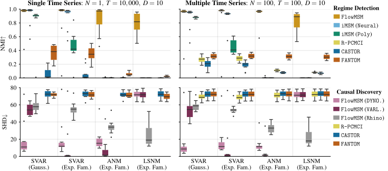
Figure 2: Performance on (top) regime detection and (bottom) causal discovery on (left) a single long time series and (right) multiple smaller time series, with $K=3$ regimes. Each boxplot covers 10 seeds.
On real-world data based on stock market indicators, our method is able to differentiate stable from volatile periods, such as the 2008 financial crisis, the COVID-19 pandemic and the early-2000s dot-com bubble. In contrast, baseline methods infer regimes and regime switches that are not easily mapped to market events. We further investigate causal interpretations of the efficient market hypothesis, among other hypotheses, but finding only partial support.
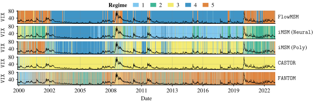
Figure 3: Estimated regimes of $\texttt{FlowMSM}$ and baseline methods on daily data of the Fama-French five-factor asset-pricing model, supplemented by excess returns of Apple's stock ($\texttt{AAPL}$), with an overlay of the $\texttt{VIX}$ volatility index (not used in training).
In the remainder of this blog post, we formally introduce structural causal models, Markov Switching Models, our identifiability theory, $\texttt{FlowMSM}$, and the experimental results. We focus on our main contribution: establishing identifiability for a broad class of regime-switching (nonlinear) structural causal models (SCMs) under independent exponential family noise. Identifiability theory here characterises when the data likelihood uniquely determines latent regimes.
The narrative below is largely based on a recent talk. For further details, we refer to the original paper.
A crash course in structural causal models (SCMs)
Let's begin with a standard definition
A structural causal model (Pearl, 2009) encodes the causal relations between
endogenous variables $\bm{X}=(X_1,\dots,X_D)\in\mathcal{X}$ (in this work continuous: $\mathcal{X}\subseteq\mathbb{R}^D$);
their causal parents $\operatorname{Pa}(X_i)\subset\bm{X}\setminus X_i$; and
exogenous noises $\bm{\epsilon}=(\epsilon_1,\dots,\epsilon_D)\in\mathcal{X}_\epsilon$ with $\bm{\epsilon}\sim p_{\bm{\epsilon}}$.
The data generating process can then be described by a set of structural equations:
Typically, we assume causal parents are acyclic, such that the structural equations are recursive.
Furthermore, assuming causal sufficiency, we exclude latent confounders between observed variables. That is, we assume all relevant variables are observed. (But we partly relax this later...)
This allows us to visualise the causal structure, defined by the causal parents, in a directed acyclic graph (DAG).
Figure 4: Example DAG with $D=3$ variables.
Now we add a temporal component
Say we observe time series $\bm{X}_{0:T}\in\mathcal{X}^{\times (T+1)}$.
In vector-notation, for (instantaneous) causal parents $\operatorname{\mathbf{Pa}}(\bm{X}_t)\subset\bm{X}_{t-1:t}$, we obtain initial equations,
(Some notation: We use superscript0 to denote mathematical objects specific to the initial time step.
Furthermore, for simplicity, causal parents are of maximum lag $L=1$, but all our results generalise.)
It is typical to assume causal stationarity, meaning functions $\bm{f}^0,\bm{f}$ and causal parents $\operatorname{\mathbf{Pa}}$ are invariant across time. (But we partly relax this later...)
Under causal stationarity, we observe a repeating causal structure.
Figure 5: Example temporal DAG with $D=3$ variables.
Finally, we introduce regime-switching
Consider time series $\bm{X}_{0:T}$ that is causally stationary only in discrete segments of time.
This is commonly modelled using discrete latent regime variables $R_t\in\mathcal{A}_K=\{1,\dots,K\}$, where $K<\infty$.
The set $\mathcal{A}_K$ is a finite subset of the countably infinite set $\mathcal{A}$, for example $\mathcal{A}=\mathbb{N}$, indexing all regimes in a particular model class.
The equations governing regimes $\bm{R}_{0:T}$ can be anything, although our identifiability theory requires that they cannot depend on $\bm{X}_{0:T}$.
(Some notation: We often write shorthand $\bm{f}_a\triangleq\bm{f}\rvert_{R_t=a}$ when we fix the regime to some value $a\in\mathcal{A}$.)
The regime-dependent causal structure is a DAG when the regime sequence is fixed.
That is, $R_t$ acts as a latent confounder for the variables $\bm{X}_t$, inducing a potentially different causal structure for each regime.
These need not be unique across regimes.
Figure 6: Example DAG given regimes $\bm{R}_{0:3}$, with coloured edges belonging to initial and window graphs (Assaad et al., 2022).
A brief overview of our assumptions
The assumptions below are standard in the causal literature, where we partly relax causal sufficiency and stationarity:
Acyclicity: Structural equations are recursive;
Conditional causal stationarity: Regimes fully govern structural changes over time;
Conditional causal sufficiency: No latent confounders within each regime;
Causal Markov & faithfulness: Conditional independency in the data $\Longleftrightarrow$ $d$-separation in the corresponding DAG.
For tractable estimation, we further assume:
The regimes $\bm{R}_{0:T}$ follow a first-order stationary Markov chain;
The mappings $\bm{f}^0_a,\bm{f}_a$ are contractive to guarantee stability.
Markov Switching Models (MSMs)
Each regime-switching SCM induces a corresponding MSM
The dynamic Bayesian network induced by a regime-switching SCM is a Markov Switching Model (Hamilton, 1989), a type of Hidden Markov Model (HMM) with autoregressive dependencies among latent regimes and observed variables.
Figure 7: An MSM is an autoregressive HMM.
Classic identifiability results for finite-state HMMs (Kruskal, 1977; Allman et al., 2009, Gassiat et al., 2016) do not trivially extend to MSMs due to the autoregressive connections between observed variables.
Each MSM is a finite mixture model
An MSM can be formulated as a finite mixture model (Frühwirth-Schnatter, 2006). That is, the joint distribution of $\bm{X}_{0:T}$ can be written as a finite mixture over $K^{T+1}$ regime sequences,
We can further factorise the mixture components into initial and transition distributions, drawn from the countably infinite distribution families $\textcolor{OkabeGreen}{\mathcal{P}^0_\mathcal{A}}$, $\textcolor{OkabeBlue}{\mathcal{P}_{\mathcal{A}}}$ (for example, Gaussian families with parameters indexed by $\mathcal{A}$),
Thus, the $K^{T+1}$ components of the mixture are drawn from the product family $\textcolor{OkabeGreen}{\mathcal{P}^0_\mathcal{A}}\otimes\textcolor{OkabeBlue}{\mathcal{P}_{\mathcal{A}}}^{\otimes T}$.
The problem of identifying latent regimes
Let's take a look at some examples of regime-switching SCMs
Let $\bm{W}_{a,0},\bm{W}_{a,1}$ be weighted adjacency matrices, where $\bm{W}_{a,0}$ is acyclic and for stability $\rho(\bm{W}_{a,0}),\rho(\bm{W}_{a,1})<1$.
(We leave out the initial equations below for brevity.)
where $\circ$ denotes the Hadamard product and $\delta>0$ is a tiny constant.
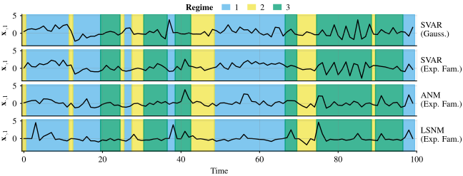
If we generate data according to these equations, then the time series might look as follows. That is, having (non-)Gaussian noise or (non)linear transitions is not necessarily easily distinguishable through visualisation.
Figure 8: The only differences between the figure rows amounts to the structural equations and exogenous noises, using (Gauss) $\epsilon_{t,d}\overset{\textit{i.i.d.}}{\sim}\mathcal{N}(0, 1)$ and (Exp. Fam.) $\epsilon_{t,d}\overset{\textit{i.i.d.}}{\sim}\text{Gamma}(0.25,2)-0.5$, both with zero mean and unit variance.
Each regime-switching SCM induces a corresponding MSM
Only for the linear SVAR with $\epsilon_{t,d}\overset{\textit{i.i.d.}}{\sim}\mathcal{N}(0, 1)$, the induced MSM is a classic Gaussian mixture model, e.g.,
$$
p_{\bm{\theta}}(\bm{x}_0\mid a) = \mathcal{N}((\bm{I}-\bm{W}_{a,0})^{-1}\bm{\mu}_a,\Sigma_a),
$$
$$
p_{\bm{\theta}}(\bm{x}_t\mid \bm{x}_{t-1}, a) = \mathcal{N}((\bm{I}-\bm{W}_{a,0})^{-1}\bm{W}_{a,1}\bm{x}_{t-1},\Sigma_a),
$$
where $\Sigma_a\triangleq (\bm{I}-\bm{W}_{a,0})^{-1}(\bm{I}-\bm{W}_{a,0})^{-T}$. Note that acyclicity guarantees invertibility of $\bm{I}-\bm{W}_{a,0}$.
It is well-known that identifiability of the mixture components (and thus the regimes) is guaranteed when the Gaussian parameters are distinct (Yakowitz and Spragins, 1968).
However, we face a problem: If
(i) instantaneous effects are not affine, or
(ii) the noise is non-Gaussian,
we no longer obtain a mixture of Gaussian distributions...
Therefore, the key question in our identifiability theory is:
When are regimes identifiable in potentially non-Gaussian mixtures?
Identifiability Theory
We start with stating our main result
MSMs are identifiable (up to permutation) if the data likelihood $p_{\bm{\theta}}(\bm{x}_{0:T})$ uniquely determines the regime prior $p_{\bm{\theta}}(\bm{r}_{0:T})$ and the mixture components $p_{\bm{\theta}}(\bm{x}_{0:T}\mid \bm{r}_{0:T})$, up to a regime relabelling.
(For brevity, we often leave out "up to permutation".)
Theorem 3.5: Identifiable Regime-Switching SCMs
Consider an acyclic regime-switching SCM that satisfies conditional causal stationarity, conditional causal sufficiency, and Ass. 3.1 to 3.4. Then the induced MSM is identifiable up to permutation.
In the remainder, we provide a proof sketch and introduce our assumptions 3.1 to 3.4.
An intermezzo on linear independence
Identifiable finite mixture distributions are characterised by the notion of linear independence.
Yakowitz & Spragins (1968)
Finite mixture distributions are identifiable if and only if the the functions in the family of mixture components are linear independent, i.e., for any finite $\mathcal{A}_K\subset\mathcal{A}$,
Thus, for our MSM setting, identifiability reduces to linear independence of the PDFs in the product family $\textcolor{OkabeGreen}{\mathcal{P}^0_\mathcal{A}}\otimes\textcolor{OkabeBlue}{\mathcal{P}_{\mathcal{A}}}^{\otimes T}$.
An initial thought could be, is linear independence in $\mathcal{P}^0_\mathcal{A}$ and $\mathcal{P}_{\mathcal{A}}$ sufficient to achieve identifiability?
Short answer: It is necessary, but not sufficient.
The reason is that an overlapping variable space challenges linear independence for any consecutive product of linearly independent distributions.
For example, for $T=1$, we have one overlapping variable $\bm{x}_0$, i.e.,
Coupling distributions through $\bm{x}_0$ might accidentally create linear dependencies in the joint variable space...
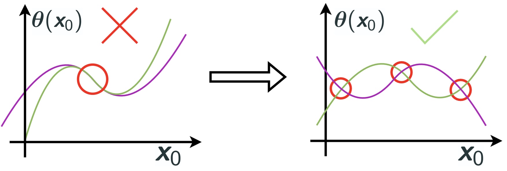
To tackle this, we rely on Balsells-Rodas et al. (2024), who propose non-parametric conditions to extend the notion of linear independence to sequences of random variables.
Their key idea is to allow linear dependence only on zero-measure subsets of the overlapping variable space. A sufficiently regular space (e.g., real-analytic) forces discontinuities to arise solely from regime changes.
Figure 9: Illustration adapted from Balsells-Rodas et al. (2024).
Hence, we obtain sufficient local conditions
If the PDFs in the initial and transition families are linearly independent, and the joint variable space is sufficiently regular, then we obtain identifiability up to permutation.
Previous work provided concrete instantiations to achieve linear independence only for multivariate Gaussian families.
Our technical contributions answer two questions:
Can we ensure linear independence in the initial and transition families beyond Gaussians?
Linear independence is an abstract notion, can we translate this to more fine-grained conditions on regime-switching SCMs?
For simplicity, we focus on the transition family, omitting the initial family.
Linear independence is further specified for exponential family distributions
Fundamentally, our proof relies on the identifiability of (finite) mixtures of exponential family distributions.
Recall, the PDF of a continuous variable $\bm{\epsilon}\in\mathcal{X}_\epsilon$ from a minimal regular exponential family is
for $P$-dimensional natural parameters $\bm{\eta}$, $P\geq 1$, sufficient statistic $\bm{\tau}$, base measure $h$ and log-partition $A$. The support $\mathcal{X}_\epsilon\subseteq\mathbb{R}^D$ does not depend on $\bm{\eta}$. The natural parameter space is open (regularity) and the sufficient statistic has linearly independent components (minimality).
Barndorff-Nielsen (1965)
(Finite) mixtures of a continuous minimal regular exponential family are identifiable if (i) the sufficient statistic is continuous with (ii) an image that contains an open set on its support.
Note the mixture is here taken over the natural parameters $\bm{\eta}$, keeping the sufficient statistic $\bm{\tau}$ and support $\mathcal{X}_\epsilon$ fixed across regimes. This will be relevant later. Finite mixtures of multivariate Gaussian families are included as a special case.
We derive conditions on regime-switching SCMs such that we can leverage Barndorff-Nielsen (1965)
We start by restricting the exogenous noise distribution.
Assumption 3.1: Exponential Family Noise
The exogenous noise $\bm{\epsilon}_t$ is from a continuous minimal regular exponential family that satisfies:
Real-analytic sufficient statistic: The sufficient statistic $\bm{\tau}$ is a real-analytic function a.e..
Rich image of the sufficient statistic: The image $\{\bm{\tau}(\bm{\epsilon}_t)\mid h(\bm{\epsilon}_t)>0,\bm{\epsilon}_t\in\mathcal{X}_\epsilon\}$ contains a (non-empty) open set.
We strengthen continuity of the sufficient statistic to real-analyticity to avoid linear dependence in the overlapping variable space.
Furthermore, the condition (a2) excludes certain degenerate and curved exponential families where the image of the sufficient statistic is confined to a lower-dimensional manifold, e.g., when $P>D$.
We aim to establish that each regime represents a unique pushforward of the noise distribution
Assumption 3.2: Functional Model Restrictions. The mappings $\bm{f}_a$ satisfy:
Unique regimes: For all $a,a'\in\mathcal{A}$, $\bm{f}_a=\bm{f}_{a'} \quad \textit{a.e.} \quad \implies \quad a=a'$;
Pointwise diffeomorphisms: For almost every $\bm{x}_{t-1}\in\mathcal{X}$, and for all $a\in\mathcal{A}$, the mapping $\bm{f}_a\rvert_{\bm{X}_{t-1}=\bm{x}_{t-1}}$ is a diffeomorphism a.e. in $\bm{\epsilon}_t$;
Jointly real-analytic transitions: For all $a\in\mathcal{A}$, the mapping $\bm{f}_a$ is jointly real-analytic in $(\bm{x}_{t-1},\bm{\epsilon}_t)$ a.e..
Condition (b3), in combination with (a1), ensures the overlapping variable space is real-analytic.
Next, we rule out some ambiguous unidentifiable cases
We rule out unidentifiable cases that exploit symmetries, e.g., rotations of isotropic Gaussians.
Assumption 3.3: Trivial Automorphisms. At least one of the following holds:
Trivial automorphisms of the noise: The noise distribution has a trivial automorphism class, i.e., for any invertible mapping $\Phi$, $\Phi(\bm{\epsilon})\overset{d}{=}\bm{\epsilon} \implies \Phi=\bm{\epsilon} \quad \textit{a.s.}$;
Monotone canonicalisation: There exists a canonical variable order s.t. $\forall a\in\mathcal{A}$, $\partial\bm{f}_a/\partial\bm{\epsilon}_t$ can be permuted to a lower-triangular matrix, and it has strictly positive diagonal a.e. in $\bm{\epsilon}_t$.
The stronger condition (c2) guarantees a unique monotone triangular transport known as the Knothe-Rosenblatt rearrangement (Knothe, 1957; Rosenblatt, 1952).
Our assumptions preserve the exponential family structure
The structural equations define mappings $\textcolor{OkabeBlue}{\Phi_a\rvert_{\bm{X}_{t-1}}=\bm{x}_{t-1}}:\mathcal{X}_\epsilon\to\mathcal{X}$ from the noise space to the observed space at each time step, for a fixed regime $a\in \mathcal{A}$.
Under Ass. 3.1-3.3, using the change of variables formula and the exponential family structure,
where $\textcolor{OkabeBlue}{\Phi^{-1}_a}(\cdot,\bm{x}_{t-1})$ denotes the inverse of $\textcolor{OkabeBlue}{\Phi_a}(\bm{x}_{t-1}, \cdot)$ with respect to $\bm{\epsilon}_t$ for fixed $\bm{x}_{t-1}$.
This is still an exponential family, but each transition distribution might have a different sufficient statistic and base measure.
How can we still leverage Barndorff-Nielsen (1965)?
A reparametrisation to an exponential family with a shared sufficient statistic
We establish a reparametrisation of $\mathcal{P}^0_{\mathcal{A}}$ and $\mathcal{P}_{\mathcal{A}}$ to an exponential family with common sufficient statistic and base measure through a finite-order polynomial factorisation. This enables known theory from Barndorff-Nielsen (1965).
Assumption 3.4: Sufficient variability across regimes in a finite polynomial subspace.
The mappings $\Phi_a$ satisfy for some finite $O<\infty$ and all $a\in\mathcal{A}$ and almost every $\bm{x}_{t-1}\in\mathcal{X}$:
Common support: The base measure $h\circ \Phi^{-1}_a$ can be separated into a common base measure $\widetilde{h}$ and a scaling function $b_a(\bm{x}_{t-1})>0$;
Finite polynomial reparametrisation: There exists a common sufficient statistic $\widetilde{\bm{\tau}}:\mathcal{X}\to\mathbb{R}^{\widetilde{P}}$, with $\widetilde{P}\geq P$, whose components are monomials up to order $O$, and matrices $\bm{C}_a(\bm{x}_{t-1})\in\mathbb{R}^{P\times\widetilde{P}}$ with full row rank $P$, such that
$$
\bm{\tau}\circ \Phi^{-1}_a(\bm{x}_t,\bm{x}_{t-1})=\bm{C}_a(\bm{x}_{t-1})\widetilde{\bm{\tau}}(\bm{x}_t) +\mathcal{R}_O(\bm{x}_t) \quad \textit{a.e.},
$$
where the remainder is regime-invariant and can be absorbed into the base measure;
Injectivity of polynomial coefficients: For all $a\neq a'\in\mathcal{A}$,
$$
\bm{C}_a(\bm{x}_{t-1})^T\bm{\eta}=\bm{C}_{a'}(\bm{x}_{t-1}) ^T\bm{\eta} \quad \forall \bm{\eta}\in\mathbb{R}^P \quad \implies \quad \Phi_a=\Phi_{a'}\quad \textit{a.e.}
$$
Intuitively, this assumption imposes sufficient variability across regimes in a finite-dimensional polynomial subspace of the sufficient statistic. That is, all regime-discriminating information is captured by a finite amount of linearly independent monomial terms, while any remaining non-polynomial components are invariant across regimes.
In the basic setting of affine transformations of Gaussian noise, the induced sufficient statistic is a quadratic polynomial, so the decomposition holds with finite dimension $\widetilde{P}=P$ and zero remainder. For nonlinear real-analytic transformations, the regime-invariant remainder enforces the absence of high-order regime signal beyond the low-order polynomial terms.
Putting it all together
Ass. 3.4 guarantees an equivalent representation as a continuous minimal regular exponential family with distinct natural parameters and common sufficient statistic. All regime- and history-dependent effects can be absorbed into parameters $\bm{\theta}:\mathcal{X}\times\mathcal{A}\to\Theta$, i.e.,
Thus, the transition distribution remains a minimal regular exponential family. The same argument holds for the initial family.
To conclude, we established finite mixtures of the initial and transition distribution families are identifiable, so the families contain linearly independent functions. Throughout, we made sure the overlapping variable space is sufficiently regular, i.e., real-analytic. This satisfies the sufficient conditions for identifiability we established earlier, and it proofs our main result.
Identifiable causal graphs
Upon identification of latent regimes, known causal theory applies to identify stationary causal graphs from the disentangled transition distributions.
For example, each window graph is identifiable up to a Markov equivalence class (MEC) of conditional independencies under faithfulness (Spirtes et al., 2000).
Alternatively, the transition distributions may correspond to a single window graph when the function class of $\bm{f}^0_a,\bm{f}_a$ is restricted (Peters et al., 2011).
$\texttt{FlowMSM}$: A framework for regime detection and regime-dependent causal discovery
Assuming access to a dataset $\big\{\bm{x}^{(n)}_{0:T}\big\}^N_{n=1}$ of $N$ i.i.d. realisations of the time series $\bm{X}_{0:T}$, $\texttt{FlowMSM}$ detects latent regimes $\bm{R}_{0:T}$, while a stationary causal method subsequently discovers window graphs $\bm{G}_{1:K}$ from clustered samples.
Figure 10: We detect latent regimes and window graphs from time series, with dependencies between regimes (red edges) and instantaneous effects between observed variables (pink edges).
Regime detection
The goal here is to obtain estimates $\widehat{p}_{\bm{\theta}}(r_t\mid \bm{x}^{(n)}_{0:T})$ of the regime posterior likelihood.
We leverage the Generalised Expectation-Maximisation (GEM) algorithm for mixture model estimation, guaranteed to converge to a local optimum of the likelihood objective (Dempster et al., 1977). The forward-backward algorithm allows efficient updates of the likelihood objective.
A neural spline flow (NSF) (Durkan et al., 2019) models the transition distributions, with shared parameters $\psi$ and regime-specific embeddings $\bm{\mathcal{E}}_{1:\widetilde{K}}$. Likewise for the initial distributions.
Figure 11: $\texttt{FlowMSM}$ parameters $\bm{\theta}=(\bm{\pi},Q, \psi^0,\psi, \bm{\mathcal{E}}^0_{1:\widetilde{K}}, \bm{\mathcal{E}}_{1:\widetilde{K}})$ in the Generalised Expectation-Maximisation (GEM) objective.
A sample splitting scheme
We assign the sequences $\bm{x}^{(n)}_{t-1:t}$, $t\in\{1,\dots,T\}$, $n\in \{1, \dots, N\}$, to the MAP regime
This creates $\widetilde{K}$ clusters with partially overlapping sliding windows.
In theory, a perfect regime assignment would lead to clusters of causally stationary windows, since the causal parents of variables $\bm{x}^{(n)}_t$ depend solely on the oracle regime $r^{(n)}_t$. In practice, we show $\texttt{FlowMSM}$ exhibits high accuracy in most settings.
Regime-dependent causal discovery
To estimate window graphs from the clustered samples, $\texttt{FlowMSM}$ can be paired with any stationary causal discovery method that allows for instantaneous effects. We use the following well-known methods:
$\texttt{VARLiNGAM}$ (Hyvärinen et al., 2010)
$\texttt{DYNOTEARS}$ (Pamfil et al., 2020)
$\texttt{PCMCI+}$ (Runge, 2020)
$\texttt{Rhino}$ (Gong et al., 2023)
Experiments
Strong performance on synthetic data
Recall the examples of regime-switching SCMs we discussed earlier (linear SVAR, nonlinear ANM, LSNM)? We generate synthetic data for each of these models and evaluate the performance of $\texttt{FlowMSM}$ with regard to several baseline methods. To evaluate the estimated regimes, we report the normalised mutual information (NMI$\uparrow$), where higher is better. For the estimated window graphs, we report the Structural Hamming Distance (SHD$\downarrow$), where lower is better.
For regime detection, in simple linear settings, our approach achieves performance comparable to Gaussian $\texttt{iMSM}$ baselines, as expected. In contrast, in nonlinear and non-Gaussian settings, $\texttt{FlowMSM}$ maintains strong performance, whereas baselines degrade substantially. This pattern is consistent across both a single long time series and a collection of shorter sequences.
For causal discovery, our approach shows strong performance contingent on the chosen discovery method. $\texttt{DYNOTEARS}$ performs well when regime changes primarily affect distribution location, while $\texttt{VARLiNGAM}$ excels in non-Gaussian settings, except the LSNM class, for which $\texttt{Rhino}$ performs the best. None of the baselines achieve competitive performance in these settings.
Figure 12: Performance on (top) regime detection and (bottom) causal discovery on (left) a single long time series and (right) multiple smaller time series, with $K=3$ regimes. Each boxplot covers 10 seeds.
The Fama-French five-factor asset-pricing model: Regime detection
Fama and French (2015) posit five risk factors that capture systemic patterns in stock returns: size, value, market risk, profitability and investment. Following Sadeghi et al. (2024), we supplement this by excess returns of Apple's stock ($\texttt{AAPL}$).
We run our method and baselines on daily data of these six variables, spanning the early 2000s to the end of 2022, for a total of 5,786 trading days, using $\widetilde{K}=5$ regimes. We do not have access to the ground truth causal graph nor regimes, so we provide a qualitative study by evaluating the estimated regimes by overlaying the $\texttt{VIX}$ volatility index, which is not used in training.
$\texttt{FlowMSM}$ identifies two dominant regimes aligned with periods of low and high market volatility, the latter including the 2008 financial crisis, the COVID-19 pandemic, and the early-2000s dot-com bubble. In contrast, other methods infer regimes and regime switches that are not easily mapped to market events.
Figure 13: Estimated regimes of $\texttt{FlowMSM}$ and baseline methods on daily data of the Fama-French five-factor asset-pricing model, supplemented by excess returns of Apple's stock ($\texttt{AAPL}$), with an overlay of the $\texttt{VIX}$ volatility index (not used in training).
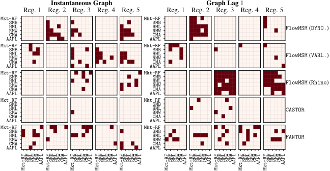
The Fama-French five-factor asset-pricing model: Regime-dependent causal discovery
Even though the Fama-French model is presented as a statistical rather than a causal model, we investigate its causal implications and limitations. For example, under the efficient market hypothesis, causal dependencies across time steps should be absent, although we expect periods of market distress may give rise to arbitrage opportunities. We only find partial support for these (and other) hypotheses, suggesting causal interpretations of the Fama-French model on this dataset are limited in scope.
Figure 14: Adjacency matrices of the window graphs corresponding to the estimated regimes. The index $(i,j,k,l)$ indicates the (lagged) edge $X_{t-l,i}\to X_{t,j}$ in regime $k$.
Some concluding remarks
We explored regime detection and causal discovery in non-stationary time series in the presence of regime switches and nonlinear and non-Gaussian dynamics. We proposed novel theory on identifiability of latent regimes under temporal regime dependencies, nonlinear lagged and instantaneous effects, and independent noise from the exponential family. Our regime detection framework, $\texttt{FlowMSM}$, readily extends to post-hoc regime-dependent causal discovery.
Our work provides a principled framework for regime identification in non-stationary time series, and we believe most of our assumptions to be reasonably mild restrictions. Future work could explore non-stationary causal models with latent confounders other than regime variables, thus further relaxing (conditional) causal sufficiency.
References
Allman, Matias, Rhodes. Identifiability of parameters in latent structure models with many observed variables. The Annals of Statistics, 2009.
Assaad, Devijver, Gaussier. Survey and evaluation of causal discovery methods for time series. Journal of Artificial Intelligence Research, 2022.
Balsells-Rodas, Wang, Li. On the identifiability of switching dynamical systems. ICML, 2024.
Dempster, Laird, Rubin. Maximum likelihood from incomplete data via the EM algorithm. Journal of the Royal Statistical Society, 1977.